Running Your First Object Detection Model on a Hailo Device Using DeGirum PySDK
This guide is for ML developers who want to learn how to configure DeGirum PySDK to load a precompiled object detection model and run inference on a Hailo device. Similar to our User Guide 1, we’ll focus on the essential details and steps involved instead of a “just run this magic two line script” approach. We encourage the readers to start with User Guide 1 before proceeding with this guide. By the end of this guide, you’ll have a solid understanding of how to work with precompiled object detection models and adapt the process to your needs.
What You’ll Need to Begin
To follow this guide, you’ll need a machine equipped with a Hailo AI accelerator, either Hailo8 or Hailo8L. The host CPU can be an x86 system or an Arm based system (like Raspberry Pi). Before diving in, make sure the necessary drivers and software tools are installed correctly. You can find the setup instructions here: Hailo + PySDK setup instructions.
Here’s what else you’ll need:
- A Model File (
.hef): This is the compiled model for Hailo hardware. We’ll be using theyolov11ndetection model, available for Hailo8 devices at Hailo8 Object Detection Models. - An Input Image: The image you want to process using the model. For this guide, we’ll use a cat image, which you can download from Cat Image.
- A Labels File (
labels_coco.json): This file maps class indices to human-readable labels for the 80 classes of COCO dataset. You can download it from Hugging Face.
Download these assets and keep them handy, as we’ll use them throughout this guide.
Summary
We’ll walk you through the steps to run inference on a Hailo device using DeGirum PySDK. Here’s what we’ll cover:
- Configuring the Model JSON File: Configure a simple model JSON file that defines key configurations for pre-processing, model parameters, and post-processing.
- Preparing the Model Zoo: Organize the model files (
.json,.hef, and labels file) for seamless use with PySDK. - Running Inference: Write Python code to load the model, preprocess the input, run inference, and process the output manually.
Configuring the Model JSON File
The model JSON file defines key configurations for the model, such as supported devices, preprocessing requirements, model paths, and postprocessing steps. Below is a simple example of a model JSON file that directly passes the input to the model and outputs raw results without additional processing. For detailed explanation of the model JSON, we refer the users to our User Guide 1.
Example: Simple Model JSON
{
    "ConfigVersion": 10,
    "DEVICE": [
        {
            "DeviceType": "HAILO8",
            "RuntimeAgent": "HAILORT",
            "SupportedDeviceTypes": "HAILORT/HAILO8"
        }
    ],
    "PRE_PROCESS": [
        {
            "InputType": "Tensor",
            "InputN": 1,
            "InputH": 640,
            "InputW": 640,
            "InputC": 3,
            "InputRawDataType": "DG_UINT8"
        }
    ],
    "MODEL_PARAMETERS": [
        {
            "ModelPath": "yolo11n.hef"
        }
    ],
    "POST_PROCESS": [
        {
            "OutputPostprocessType": "None"
        }
    ]
}
Preparing the Model Zoo
We will now organize the model assets to form a model zoo. Choose a directory where you want to store all the assets for your models.
- Copy the JSON configuration example above into a file named
yolo11n.json. - Place the corresponding
yolo11n.heffile in the same directory. - Place the labels file
coco_labels.jsonin the same directory.
If you prefer to organize models into separate directories for easier maintenance, you can create a dedicated directory for each model and store its assets there. PySDK will automatically search for model JSON files in all sub-directories of the specified zoo_url.
Running Inference
The yolo11n model takes a UINT8 array of size [1, 640, 640, 3] as input and outputs a FP32 array of size [1, 40080] (we will explain the output format later in the guide). Let’s start with some utility functions that help analyze, handle, and visualize images.
Utility Functions For Image Handling
Function to read an image from a file and returning an array in RGB format
import cv2

def read_image_as_rgb(image_path):
    # Load the image in BGR format (default in OpenCV)
    image_bgr = cv2.imread(image_path)

    # Check if the image was loaded successfully
    if image_bgr is None:
        raise ValueError(f"Error: Unable to load image from path: {image_path}")

    # Convert the image from BGR to RGB
    image_rgb = cv2.cvtColor(image_bgr, cv2.COLOR_BGR2RGB)

    return image_rgb
Function to print the height and width of an image
import cv2

def print_image_size(image_path):
    # Load the image
    image = cv2.imread(image_path)

    # Check if the image was loaded successfully
    if image is None:
        print(f"Error: Unable to load image from path: {image_path}")
    else:
        # Get the image size (height, width, channels)
        height, width, channels = image.shape
        print(f"Image size: {height}x{width} (Height x Width)")
Function to display an RGB image array
import matplotlib.pyplot as plt
def display_images(images, title="Images", figsize=(15, 5)):
    """
    Display a list of images in a single row using Matplotlib.

    Parameters:
    - images (list): List of images (NumPy arrays) to display.
    - title (str): Title for the plot.
    - figsize (tuple): Size of the figure.
    """
    num_images = len(images)
    fig, axes = plt.subplots(1, num_images, figsize=figsize)
    if num_images == 1:
        axes = [axes]  # Make it iterable for a single image
    for ax, image in zip(axes, images):
        ax.imshow(image)
        ax.axis('off')
    fig.suptitle(title, fontsize=16)
    plt.tight_layout()
    plt.show()
Preparing the Input
Let us start by looking at the input image. The code below prints the image size and displays the image.
image_path='<path to cat image>'
print_image_size(image_path)
original_image_array = read_image_as_rgb(image_path)
display_images([original_image_array], title="Original Image")
Running the code produces the output below:
Image size: 852x996 (Height x Width)
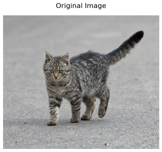
Given that the image under consideration has a size of 852 x 996 and the model requires an input of 640 x 640, the image needs to be resized to fit the model’s input size. There are different ways to resize an image to a target size, such as stretching, cropping, or padding.
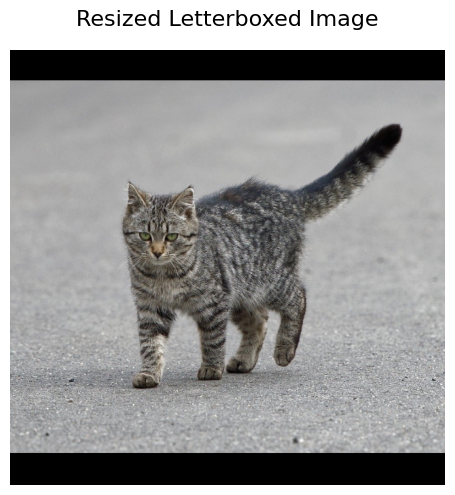
Letterboxing is commonly used in object detection models to resize input images while maintaining their original aspect ratio. The image is resized to fit within the target dimensions, and any remaining space is filled with padding. This ensures that the image content remains undistorted, which is crucial for accurate object detection. By preserving the aspect ratio, letterboxing allows the model to process images at a consistent size without losing important details or introducing distortions.
The resize_with_letterbox function resizes an image to fit a target size while preserving its aspect ratio by adding padding where necessary. It returns the resized image with padding, the scaling ratio applied to the original image, and the padding applied to the top and left sides. We will use the scale and padding values later in the guide to correctly map the bounding boxes back to the original image size.
import cv2
import numpy as np

def resize_with_letterbox(image_path, target_shape, padding_value=(0, 0, 0)):
    """
    Resizes an image with letterboxing to fit the target size, preserving aspect ratio.

    Parameters:
        image_path (str): Path to the input image.
        target_shape (tuple): Target shape in NHWC format (batch_size, target_height, target_width, channels).
        padding_value (tuple): RGB values for padding (default is black padding).

    Returns:
        letterboxed_image (ndarray): The resized image with letterboxing.
        scale (float): Scaling ratio applied to the original image.
        pad_top (int): Padding applied to the top.
        pad_left (int): Padding applied to the left.
    """
    # Load the image from the given path
    image = cv2.imread(image_path)

    # Check if the image was loaded successfully
    if image is None:
        raise ValueError(f"Error: Unable to load image from path: {image_path}")

    # Convert the image from BGR to RGB
    image = cv2.cvtColor(image, cv2.COLOR_BGR2RGB)

    # Get the original image dimensions (height, width, channels)
    h, w, c = image.shape

    # Extract target height and width from target_shape (NHWC format)
    target_height, target_width = target_shape[1], target_shape[2]

    # Calculate the scaling factors for width and height
    scale_x = target_width / w
    scale_y = target_height / h

    # Choose the smaller scale factor to preserve the aspect ratio
    scale = min(scale_x, scale_y)

    # Calculate the new dimensions based on the scaling factor
    new_w = int(w * scale)
    new_h = int(h * scale)

    # Resize the image to the new dimensions
    resized_image = cv2.resize(image, (new_w, new_h),interpolation=cv2.INTER_LINEAR)

    # Create a new image with the target size, filled with the padding value
    letterboxed_image = np.full((target_height, target_width, c), padding_value, dtype=np.uint8)

    # Compute the position where the resized image should be placed (padding)
    pad_top = (target_height - new_h) // 2
    pad_left = (target_width - new_w) // 2

    # Place the resized image onto the letterbox background
    letterboxed_image[pad_top:pad_top+new_h, pad_left:pad_left+new_w] = resized_image

    final_image = np.expand_dims(letterboxed_image, axis=0)

    # Return the letterboxed image, scaling ratio, and padding (top, left)
    return final_image, scale, pad_top, pad_left
We can use the above function to preprocess the image and visualize the input to model.
image_array, scale, pad_top, pad_left = resize_with_letterbox('<path to cat image>', (1, 640,640,3))
display_images([image_array[0]])
Running the above code results in the output below:
Running the Model Predict Function
Now let’s load the model, prepare the input image, and run inference:
import degirum
from pprint import pprint

# Load the model
model = dg.load_model(
    model_name='yolo11n',
    inference_host_address='@local',
    zoo_url='<path_to_model_zoo>'
)

# Prepare the input image
image_array, scale, pad_top, pad_left = resize_with_letterbox('<path_to_cat_image>', model.input_shape[0])

# Run inference
inference_result = model(image_array)

# Pretty print the results
pprint(inference_result.results)
Interpreting the Results
The inference_result is of type degirum.postprocessor.InferenceResults. For now, we focus on inference_result.results, which is a list of dictionaries. Here’s how the output looks like:
[{'data': array([[ 0.0000000e+00,  0.0000000e+00,  0.0000000e+00, ...,
         4.5914945e-41, -2.2524713e+12,  4.5914945e-41]], dtype=float32),
  'id': 0,
  'name': 'yolov11n/yolov8_nms_postprocess',
  'quantization': {'axis': -1, 'scale': [1], 'zero': [0]},
  'shape': [1, 40080],
  'size': 40080,
  'type': 'DG_FLT'}]
The output of yolo11n object detection model on Hailo is an array of size 40,080, designed to handle up to 100 detections per class across 80 classes. Each detection contains 5 values: 4 for the bounding box coordinates (ymin, xmin, ymax, xmax) and 1 for the score. The array starts with an entry that specifies the number of detections for a class. If the number is zero, it indicates no detections for that class. If there are detections for a class, the next 5 k entries represent the information for those k detections, where each detection is described by its 4 bounding box coordinates and score. This structure allows for a maximum of 100 detections per class, and the total size of the array is 40,080 (501 entries for each of the 80 classes). While the Hailo model already has an in built postprocessor that performs bounding box decoding and non-max suppression (NMS), the above input still needs to be processed so that it results in a human readable format.
Post-Processing
The postprocess_detection_results function processes the raw output tensor from an object detection model and formats the results into a structured list of dictionaries.
Explanation:
-
Parameters:
detection_output: A tensor containing the raw detection results (e.g., bounding box coordinates, confidence scores).input_shape: The shape of the input image (helps in scaling bounding boxes back to the image size).num_classes: The number of object classes that the model can predict.label_dictionary: A mapping of class IDs to human-readable labels.confidence_threshold: A minimum threshold for confidence scores. Detections below this threshold are discarded.
-
Process:
- The function first unpacks the input shape and reshapes the
detection_outputto process it. - It iterates through each class ID to parse the detections for that class.
- For each detection, it extracts the bounding box coordinates and the confidence score.
- If the confidence score is below the threshold, the detection is skipped.
- The bounding box coordinates are scaled back to the original image size based on the input dimensions.
- Each valid detection is stored in a dictionary with the bounding box, score, class ID, and label.
- If no further detections are found, the loop terminates early.
- The function first unpacks the input shape and reshapes the
-
Returns:
- A list of dictionaries, each containing a bounding box, confidence score, class ID, and label for each valid detection.
This function helps in converting raw model outputs into a format suitable for further analysis or visualization, such as drawing bounding boxes on an image.
def postprocess_detection_results(detection_output, input_shape, num_classes, label_dictionary, confidence_threshold=0.3):
    """
    Process the raw output tensor to produce formatted detection results.

    Parameters:
        detection_output (numpy.ndarray): The flattened output tensor from the model containing detection results.
        input_shape (tuple): The shape of the input image in the format (batch, input_height, input_width, channels).
        num_classes (int): The number of object classes that the model predicts.
        label_dictionary (dict): Mapping of class IDs to class labels.
        confidence_threshold (float, optional): Minimum confidence score required to keep a detection. Defaults to 0.3.

    Returns:
        list: List of dictionaries containing detection results in JSON-friendly format.
    """
    # Unpack input dimensions (batch is unused, but included for flexibility)
    batch, input_height, input_width, _ = input_shape

    # Initialize an empty list to store detection results
    new_inference_results = []

    # Reshape and flatten the raw output tensor for parsing
    output_array = detection_output.reshape(-1)

    # Initialize an index pointer to traverse the output array
    index = 0

    # Loop through each class ID to process its detections
    for class_id in range(num_classes):
        # Read the number of detections for this class from the output array
        num_detections = int(output_array[index])
        index += 1  # Move to the next entry in the array

        # Skip processing if there are no detections for this class
        if num_detections == 0:
            continue

        # Iterate through each detection for this class
        for _ in range(num_detections):
            # Ensure there is enough data to process the next detection
            if index + 5 > len(output_array):
                # Break to prevent accessing out-of-bounds indices
                break

            # Extract confidence score and bounding box values
            score = float(output_array[index + 4])
            y_min, x_min, y_max, x_max = map(float, output_array[index : index + 4])
            index += 5  # Move index to the next detection entry

            # Skip detections if the confidence score is below the threshold
            if score < confidence_threshold:
                continue

            # Convert bounding box coordinates to absolute pixel values
            x_min = x_min * input_width
            y_min = y_min * input_height
            x_max = x_max * input_width
            y_max = y_max * input_height

            # Create a detection result with bbox, score, and class label
            result = {
                "bbox": [x_min, y_min, x_max, y_max],  # Bounding box in pixel coordinates
                "score": score,  # Confidence score of the detection
                "category_id": class_id,  # Class ID of the detected object
                "label": label_dictionary.get(str(class_id), f"class_{class_id}"),  # Class label or fallback
            }
            new_inference_results.append(result)  # Store the formatted detection

        # Stop parsing if remaining output is padded with zeros (no more detections)
        if index >= len(output_array) or all(v == 0 for v in output_array[index:]):
            break

    # Return the final list of detection results
    return new_inference_results
We can run the code snippet below that utilizes the above postprocessing function to get the detection results in an easy to understand format.
import json
with open('<path to labels json file>', "r") as json_file:
    label_dictionary = json.load(json_file)
detection_results = postprocess_detection_results(inference_result.results[0]['data'], model.input_shape[0], 80, label_dictionary)
pprint(detection_results)
The output looks as below:
[{'bbox': [163.3024787902832,
           106.84022903442383,
           577.5683212280273,
           500.5242919921875],
  'category_id': 15,
  'label': 'cat',
  'score': 0.8902369737625122}]
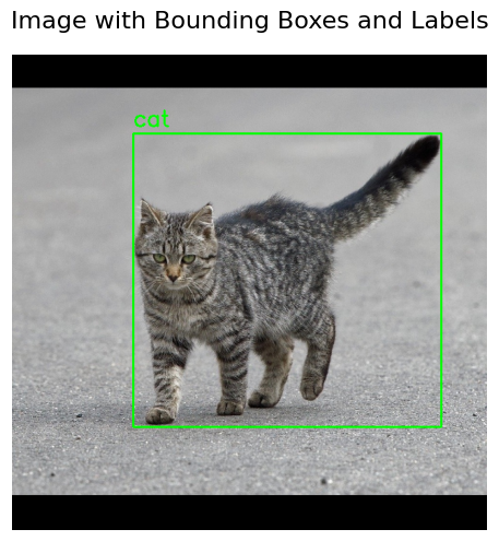
Output Visualization
As we can see, the result says that there is a cat in the image and it also provides the bounding box coordinates. We can use the function below to visualize the bounding box to confirm that the cat has been detected at the right place.
The overlay_bboxes_and_labels function overlays bounding boxes and labels on an input image.
Explanation:
-
Parameters:
image (ndarray): The input image in RGB format that will have bounding boxes and labels drawn on it.annotations (list of dicts): A list of annotations, where each annotation contains:'bbox': A tuple of bounding box coordinates(x1, y1, x2, y2)that specify the top-left and bottom-right corners of the box.'label': The text label to display for the detected object.
color (tuple): The color of the bounding box and label text (default is green(0, 255, 0)).font_scale (int): The font scale for the label text (default is1).thickness (int): The thickness of the bounding box and text (default is2).
-
Process:
- Convert image color: The input image is converted from RGB to BGR format, as OpenCV uses BGR by default for color operations.
- Loop over annotations: The function loops over each annotation (bounding box and label) in the provided list:
- It extracts the bounding box coordinates (
x1,y1,x2,y2) and label. - The coordinates are rounded and converted to integers, as OpenCV requires integer values for drawing bounding boxes.
- It extracts the bounding box coordinates (
- Draw bounding box: The bounding box is drawn using
cv2.rectangle(), which draws a rectangle using the top-left and bottom-right corners. The rectangle’s color and thickness are specified. - Add label text: The label text is placed on the image just above the bounding box using
cv2.putText(). The position, font, color, and thickness of the text are specified. - Convert back to RGB: After drawing the bounding boxes and labels, the image is converted back from BGR to RGB for further processing or display.
-
Returns:
- The image with the bounding boxes and labels overlaid, in RGB format.
import cv2
import numpy as np

def overlay_bboxes_and_labels(image, annotations, color=(0, 255, 0), font_scale=1, thickness=2):
    """
    Overlays bounding boxes and labels on the image for a list of annotations.

    Parameters:
        image (ndarray): The input image (in RGB format).
        annotations (list of dicts): List of dictionaries with 'bbox' (x1, y1, x2, y2) and 'label' keys.
        color (tuple): The color of the bounding box and text (default is green).
        font_scale (int): The font scale for the label (default is 1).
        thickness (int): The thickness of the bounding box and text (default is 2).

    Returns:
        image_with_bboxes (ndarray): The image with the bounding boxes and labels overlayed.
    """
    # Convert the image from RGB to BGR (OpenCV uses BGR by default)
    image_bgr = cv2.cvtColor(image, cv2.COLOR_RGB2BGR)

    # Loop over each annotation (bbox and label)
    for annotation in annotations:
        bbox = annotation['bbox']  # Bounding box as (x1, y1, x2, y2)
        label = annotation['label']  # Label text

        # Unpack bounding box coordinates
        x1, y1, x2, y2 = bbox

        # Convert float coordinates to integers
        x1, y1, x2, y2 = int(round(x1)), int(round(y1)), int(round(x2)), int(round(y2))

        # Draw the rectangle (bounding box)
        cv2.rectangle(image_bgr, (x1, y1), (x2, y2), color, thickness)

        # Put the label text on the image
        cv2.putText(image_bgr, label, (x1, y1 - 10), cv2.FONT_HERSHEY_SIMPLEX, font_scale, color, thickness)

    # Convert the image back to RGB for display or further processing
    image_with_bboxes = cv2.cvtColor(image_bgr, cv2.COLOR_BGR2RGB)

    return image_with_bboxes
We can run the code snippet below to visualize the results:
overlay_image = overlay_bboxes_and_labels(image_array[0], detection_results)
display_images([overlay_image], title="Image with Bounding Boxes and Labels")
The output looks as below confirming that the model predicted the bounding box correctly.
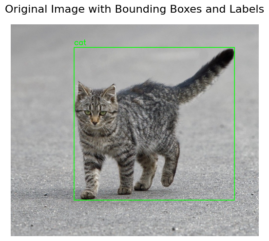
Scaling the Results to Original Image
The visualization in the previous step was with respect to the input to the detection model. However, in the application code, we would like to visualize the results with respect to the original image. We can use the function below to rescale the detections to original image size by using the scale and padding information from the preprocessing step.
def reverse_rescale_bboxes(annotations, scale, pad_top, pad_left, original_shape):
    """
    Reverse rescales bounding boxes from the letterbox image to the original image, returning new annotations.

    Parameters:
        annotations (list of dicts): List of dictionaries, each containing a 'bbox' (x1, y1, x2, y2) and other fields.
        scale (float): The scale factor used for resizing the image.
        pad_top (int): The padding added to the top of the image.
        pad_left (int): The padding added to the left of the image.
        original_shape (tuple): The shape (height, width) of the original image before resizing.

    Returns:
        new_annotations (list of dicts): New annotations with rescaled bounding boxes adjusted back to the original image.
    """
    orig_h, orig_w = original_shape  # original image height and width

    new_annotations = []

    for annotation in annotations:
        bbox = annotation['bbox']  # Bounding box as (x1, y1, x2, y2)

        # Reverse padding
        x1, y1, x2, y2 = bbox
        x1 -= pad_left
        y1 -= pad_top
        x2 -= pad_left
        y2 -= pad_top

        # Reverse scaling
        x1 = int(x1 / scale)
        y1 = int(y1 / scale)
        x2 = int(x2 / scale)
        y2 = int(y2 / scale)

        # Clip the bounding box to make sure it fits within the original image dimensions
        x1 = max(0, min(x1, orig_w))
        y1 = max(0, min(y1, orig_h))
        x2 = max(0, min(x2, orig_w))
        y2 = max(0, min(y2, orig_h))

        # Create a new annotation with the rescaled bounding box and the original label
        new_annotation = annotation.copy()
        new_annotation['bbox'] = (x1, y1, x2, y2)

        # Append the new annotation to the list
        new_annotations.append(new_annotation)

    return new_annotations
Running the code snippet below scales the detections back to original image size and shows the results overlaid on original image.
scaled_detections = reverse_rescale_bboxes(detection_results, scale, pad_top, pad_left,original_image_array.shape[:2])
overlay_original_image = overlay_bboxes_and_labels(original_image_array, scaled_detections)
display_images([overlay_original_image], title="Original Image with Bounding Boxes and Labels")
The final result looks as below:
You can try the final code with different images to assess the quality of the model. You can replace the model with any other precompiled model that has the same output format.
Conclusion
In this guide, we’ve walked through the steps of setting up and running an object detection model on a Hailo device using DeGirum PySDK. From understanding the model configuration and preparing input data to running inference and post-processing the results, you’ve gained a comprehensive overview of how to work with precompiled models in PySDK. By following these steps, you can easily integrate object detection into your applications, visualize the results, and fine-tune the process for your specific use cases. In the next guide, we will show how to use the built-in features in PySDK to simplify this whole process, enabling you to achieve the same result with just three lines of code.